
Pyspark
Overview
- speed up or scale up, Throughput or Response time
- parallel time
- skewness degree
- Shared-Something Architecture: A mixture of shared-memory and shared-nothing architectures
- Round-robin or random equal data partitioning, Hash data partitioning, Range data partitioning, Random-unequal data partitioning
- Round-robin or random equal data partitioning is “Equal partitioning” or “Random-equal partitioning”, Data evenly distributed
- Hash data partitioning (not balanced) uses A hash function
- Range data partitioning (not balanced) Spreads the records based on a given range
- Complex Data Partitioning: Complex data partitioning is based on multiple attributes or is based on a single attribute but with multiple partitioning methods. Hybrid-Range Partitioning Strategy (HRPS), Multiattribute Grid Declustering (MAGIC), Bubba’s Extended Range Declustering (BERD)
- Serial search algorithms: Linear search and Binary search
- Parallel search algorithms: Processor activation or involvement, Local searching method and Key comparison
- Depends on the data partitioning method used, Also depends on what type of selection query is performed (P15)
- Depends on the data ordering, regarding the type of the search
- Depends on whether the data in the table is unique or not
- Parallel Inner Join components
- Data Partitioning
- Divide and Broadcast
- Disjoint Partitioning
- Local Join
- Nested-Loop Join
- Sort-Merge Join
- Hash Join, The records of files R and S are both hashed to the same hash file, using the same hashing function on the join attributes A of R and B of S as hash keys
- (P23/27,28, Important) Example of a Parallel Inner Join Algorithm
- Divide and Broadcast, plus Hash Join
- data partitioning using the divide and broadcast method, and a local join
- Divide one table into multiple disjoint partitions, where each partition is allocated a processor, and broadcast the other table to all available processors
- Dividing one table can simply use equal division
- Broadcast means replicate the table to all processors
- Hence, choose the smaller table to broadcast and the larger table to divide
- (*P30) Parallel Join Query Processing
- ROJA (Redistribution Outer Join Algorithm)
- DOJA (Duplication Outer Join Algorithm)
- DER (Duplication & Efficient Redistribution)
- OJSO (Outer Join Skew Optimization)
- Serial Sorting – INTERNAL, The data to be sorted fits entirely into the main memory: Bubble Sort, Insertion Sort, Quick Sort. Serial Sorting - EXTERNAL The data to be sorted DOES NOT fit entirely into the main memory: Sort-Merge
- Parallel External Sort
- Parallel Merge-All Sort, local sort and final merge, Heavy load on one processor
- Parallel Binary-Merge Sort, Merging in pairs only, merging is still heavy
- Parallel Redistribution Binary-Merge Sort, add Redistribution, height of the tree.
- Parallel Redistribution Merge-All Sort, Reduce the height of the tree, and still maintain parallelism, Skew problem in the merging
- Parallel Partitioned Sort, Partitioning stage (Round Robin) and Independent local work, Skew produced by the partitioning.
- Parallel Group By, (Merge-All and Hierarchical Merging), Two-phase method, and Redistribution method
- Two-phase method: local records according to the groupby attribute, global aggregation where all temp results from each processor are redistributed
- Redistribution Method: redistribute raw records to all processors and each processor performs a local aggregation.
- Featurization-Extraction
- Count Vectorizer
- TF-IDF * (important)
- Word2Vec
- Featurization-Transformation
- Tokenization
- Stop Words Remover
- String Indexing
- One Hot Encoding
- Vector Assembler
- Featurization-Selection
- Vector Slicer
- Supervised Machine Learning: Classification and
Regression.
- Decision Trees (* P55) p(x)log(1/p(x))
- Compute the entropy for data set
- For every attribute/feature: 2.1. Calculate entropy for all categorical values 2.2 Take average information entropy for the current attribute 2.3 Calculate gain for the current attribute
- Pick the highest gain attribute
- Repeat until the tree is complete
- Unsupervised Machine Learning: Clustering
- K-Means clustering (P76)
- data parallelism and result parallelism
- Collaboration Filtering (P87)
- Data collection: Collecting user behaviour and associated data items
- Data processing: Processing the collected data
- Recommendation Calculation: The recommended calculation method used to calculate referrals
- Derive the result: Extract the similarity, sort it, and extract the top N to complete
- Joins In Data Streams
- Symmetric Hash Join, similer to hash join but within the window.
- M Join - M-ways Hash Join
- AM Join - add a BiHT based on M join
- Handshake Join
- Granularity Reduction
- Granularity is the level of detail at which data are stored in a database.
- Temporal-based Mixed Levels of Granularity
- Time based. - Spatial-based Mixed Levels of Granularity
- Space or location based.
- add new dimension to the observation, and hence it helps to estimate more parameters
- Multiple sensors measuring the same things
- Reduce and then Merge
- Merge and then Reduce - Multiple sensors measuring different things, but they are grouped together.
- Reduce, Normalize, and then Merge
- Normalize, Merge and then Reduce
trends
- Python as the base programming language
- Apache Kafka
- Apache Spark and Streaming
features of Big Data
- Volume: Parallel Algorithms, MapReduce
- Complexity: Machine learning algorithms, Spark MLlib enhances machine learning because of its simplicity, scalability, and easy integration with other tools.
- Classification
- Regression
- Clustering
- Velocity
- High speed data
- High inaccuracy
- Needs some pre-processing
- How to filter data
- How to pre-process data
- How to store data
Objectives
- Throughput: the number of tasks that can be completed within a given time interval
- Response time: the amount of time it takes to complete a single task from the time it is submitted
- Speed up: Performance improvement gained because of extra processing elements added, Running a given task in less time by increasing the degree of parallelism
- Scale up: Handling of larger tasks by increasing the degree of parallelism. The ability to process larger tasks in the same amount of time by providing more resources.
Volume
- Speed up and overhead
- Skew and Load balancing
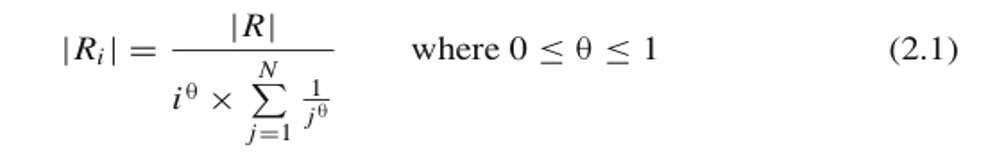
- The symbol $\theta$ denotes the degree of skewness, where $\theta$= 0 indicates no skew, and $\theta$= 1 indicates highly skewed
-
R is number of records in the table, Ri is number of records in processor i, and N is number of processor (j is a loop counter, starting from 1 to N)
- database
- Interquery parallelism: Different queries or transactions are executed in parallel with one another
- Intraquery parallelism: Execution of a single query in parallel on multiple processors and disks
- Interoperation parallelism: Speeding up the processing of a query by parallelizing the execution of each individual operation (e.g. parallel sort, parallel search, etc)
- Intraoperation parallelism: Parallelism due to the data being partitioned (Pipeline parallelism and Independent parallelism)
- Mixed parallelism
- Parallel Database Architectures
- Shared-memory architecture
- Shared-disk architecture
- Shared-nothing architecture: Each processor has its own local main memory and disks, Load balancing becomes difficult
- Shared-something architecture
- data partition
- Vertical vs. Horizontal data partitioning
- Round-robin data partitioning
- Hash data partitioning
- Range data partitioning
- Random-unequal data partitioning
Basic data partitioning is based on a single attribute (or no attribute). Complex data partitioning is based on multiple attributes or is based on a single attribute but with multiple partitioning methods
-
Hybrid-Range Partitioning Strategy (HRPS), Partitions the table into many fragments using range, and the fragments are distributed to all processors using round-robin
-
Multiattribute Grid Declustering, Based on multiple attributes - to support search queries based on either of data partitioning attributes
- Search
- Linear Search
- Binary Search
- Parallel search algorithms
- Key comparison
Join
- Nested loop join algorithm
- Sort-merge join algorithm
-
Hash-based join algorithm
-
Parallel join algorithms have two stages: Data partitioning and Local join.
- Two types of data partitioning: Divide and broadcast and Disjoint partitioning
Parallel Outer Join processing methods
- ROJA (Redistribution Outer Join Algorithm)
- DOJA (Duplication Outer Join Algorithm)
- DER (Duplication & Efficient Redistribution)
Load Balancing
- OJSO (Outer Join Skew Optimization)
Parallel Sort and GroupBy
Example
- File size to be sorted = 108 pages, number of buffer (or memory size) = 5 pages Number of subfiles = 108/5 = 22 subfiles (the last subfile is only 3 pages long).
- Pass 0 (sorting phase): For each subfile, read from disk, sort in main-memory, and write to disk (Note: sorting the data in main-memory can use any fast in-memory sorting method, like Quick Sort)
- Merging phase: We use B-1 buffers (4 buffers) for input and 1 buffer for output
- Pass 1: Read 4 sorted subfiles and perform 4-way merging (apply a need k-way algorithm). Repeat the 4-way merging until all subfiles are processed. Result = 6 subfiles with 20 pages each (except the last one which has 8 pages)
- Pass 2: Repeat 4-way merging of the 6 subfiles like pass 1 above. Result = 2 subfiles
-
Pass 3: Merge the last 2 subfiles
- Parallel Merge-All Sort, Heavy load on one processor Network contention
- Parallel Binary-Merge Sort, Merging work is now spread to pipeline of processors, but merging is still heavy
- Parallel k-way merging, k-way merging requires k files open simultaneously
- Parallel Redistribution Binary-Merge Sort, The advantage is true parallelism in merging. Skew problem in the merging
- Parallel Partitioned Sort, Partitioning (or range redistribution) may raise load skew, Local sort is done after the partitioning, not before. No merging is necessary. Main problem: Skew produced by the partitioning
Parallel GroupBy
- Traditional methods (Merge-All and Hierarchical Merging)
- Two-phase method
- Redistribution method
- Two-phase and Redistribution methods perform better than the traditional and hierarchical merging methods
- Two-phase method works well when the number of groups is small, whereas the Redistribution method works well when the number of groups is large
Machine Learning
- All learning algorithms require defining a set of features for each item, defining the right features is the most challenging part of using machine learning.
- Two types of supervised machine learning: Classification and Regression.
- Precision : measures the % of the correct classification from the predicted members: true positives / (true positives + false positives)
- Recall : measures the % of the correct classification from the overall members: true positives / (true positives + false negatives)
- F1 : measures the balances of precision and recall: 2((precisionrecall) / (precision + recall))
- Extraction : Extracting features from “raw” data, Count Vectorizer, Word2Vec,
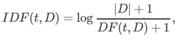
- TF-IDF, Denote a term by t, a document by d, and the corpus by D. Term frequency TF(t,d) is the number of times that term t appears in document d, while document frequency DF(t,D) is the number of documents that contains term t. where |D| is the total number of documents in the corpus.
TF-IDF measure is simply the product of TF and IDF:
- Transformation : Scaling, converting, or modifying features. Tokenization, Stop Words Remover, String Indexing, One Hot Encoding, Vector Assembler (Implement In tutorial)
- Selection : Selecting a subset from a larger set of features
Classification Algorithms (PPT 6)
- Decision Tree, The algorithm creates a multiway tree, finding for each node (i.e. in a greedy manner) the categorical feature that will yield the largest information gain for categorical targets.
- Random Forest
- DEMO
- Binary classifier
-
Multi-Class classifiers
-
Decision Tree: Might suffer from overfitting. Does not easily work with non-numerical data. Low prediction accuracy for a dataset in comparison with other machine learning classification algorithms. When there are many class labels, calculations can be complex.
- Supervised learning: discover patterns in the data that relate to data attributes with a target (class) attribute. These patterns are then utilized to predict the values of the target attribute in future data instances.
-
Unsupervised learning: The data have no target attribute.
- Key factor in clustering is the similarity measure via Euclidean Distance
- The k-means algorithm partitions the given data into k clusters. Each cluster has a cluster center, called centroid
-
Pros, Simple and fast for low dimensional data (time complexity of K Means is linear i.e. O(n)). Scales to large data sets Easily adapts to new data points
- Cons, It will not identify outliers. Restricted to data which has the notion of a centre (centroid)
how to choose k
- Elbow Method: Sum of squared errors as a function of k (a scree plot)
- Silhouette analysis : Measure of how close each point in one cluster is to points in the neighbouring clusters and thus provides a way to assess number of clusters.
Recommender System
- Content based
- Collaborative Filtering: Recommend items with the most similar items. Euclidean distance and Pearson correlation, calculation point
Streaming Computing
- Popular approach: windowing Query processing is performed only on the tuples inside the window.
- Window types: Time-based and Tuple-based (count-based)
- Event time: the time when the data is produced by the source.
- Processing time: the time when data is arrived at the processing server.
- In ideal situation, event time = processing time. In real world event time is earlier than the processing time due to network delay.The delay can be uniformed (ideal situation) or non-uniform (most of real network situation). Data may arrive in “burst” (bursty network).
Database VS. Streamming
Database
- Bounded data.
- Relatively static data
- Complex, ad-hoc query
- Possible to backtrack during processing
- Exact answer to a query
- Tuples arrival rate is low
Stream
- Unbounded data.
- Dynamic data.
- Simple, continuous query
- No backtracking, single pass operation.
- Approximate answer to a query
- Tuples arrival rate is high
Kafka
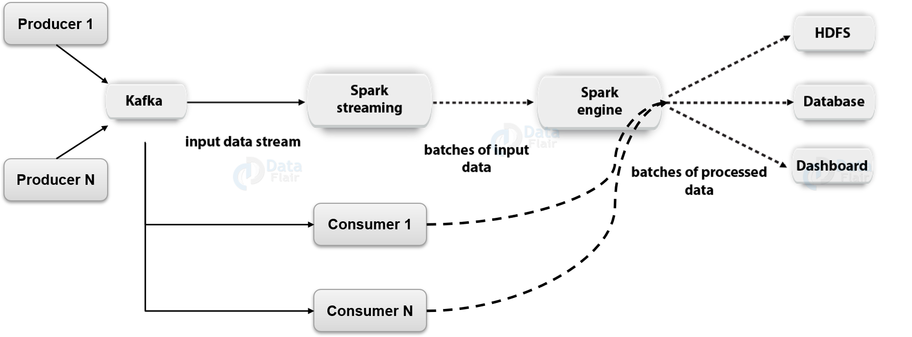
- All messages are persisted and replicated to peer brokers for fault tolerance
-
Log data structure
- Plotting Graphs: What to do if the data does not fit in the main memory? Sampling
Stream join
stream join is based on the data in the current window
- Overlapped Windows, Slide time is less than the window size
- Non-overlapped Windows, Slide time is equivalent to the window size
Two categories:
- Multiple sensors measuring the same things, and
- Multiple sensors measuring different things, but they are grouped together.
Two methods to lower the granularity of sensor arrays that measure the different thing:
- Method 1: Reduce, Normalize, and then Merge
- Method 2: Normalize, Merge and then Reduce
The normalisation process is to convert the raw data into a category, which binds different sensors into one common thread.